Cluster 2d surface to create polygons for DSeries models

In this tutorial the process of the 2d surface clustering is explained. This refers to the Datafusiontools.d_series_parser.clustering.ClusteringLayers class. The user can cluster a list of point with a certain value by using the method Datafusiontools.d_series_parser.clustering.ClusteringLayers.cluster_2d_surface().

In this tutorial we will go through the steps followed internally by this method. We start with an example surface of a dike segment and the IC value. As it is seen in the figure that follows

Step 1: Call from the user

The user calls the clustering function as follows:

cluster_model = ClusteringLayers()
cluster_model.cluster_2d_surface(points_2d_slice,
                                     k_candidates=4,
                                     cluster_variables=["value"],
                                     spatial_connectivity_methods=libpysal.weights.Queen)

Step 2: Normalizing the data

All data points and value are normalised by the function Datafusiontools.d_series_parser.clustering.ClusteringLayers.normalise_data() .

Step 3: Clustering with the Spatially Constrained Hierarchical Clustering method

At this point the clustering method begins based on the Spatially Constrained Hierarchical Clustering method. More on that method can be read on https://geographicdata.science/book/notebooks/10_clustering_and_regionalization.html

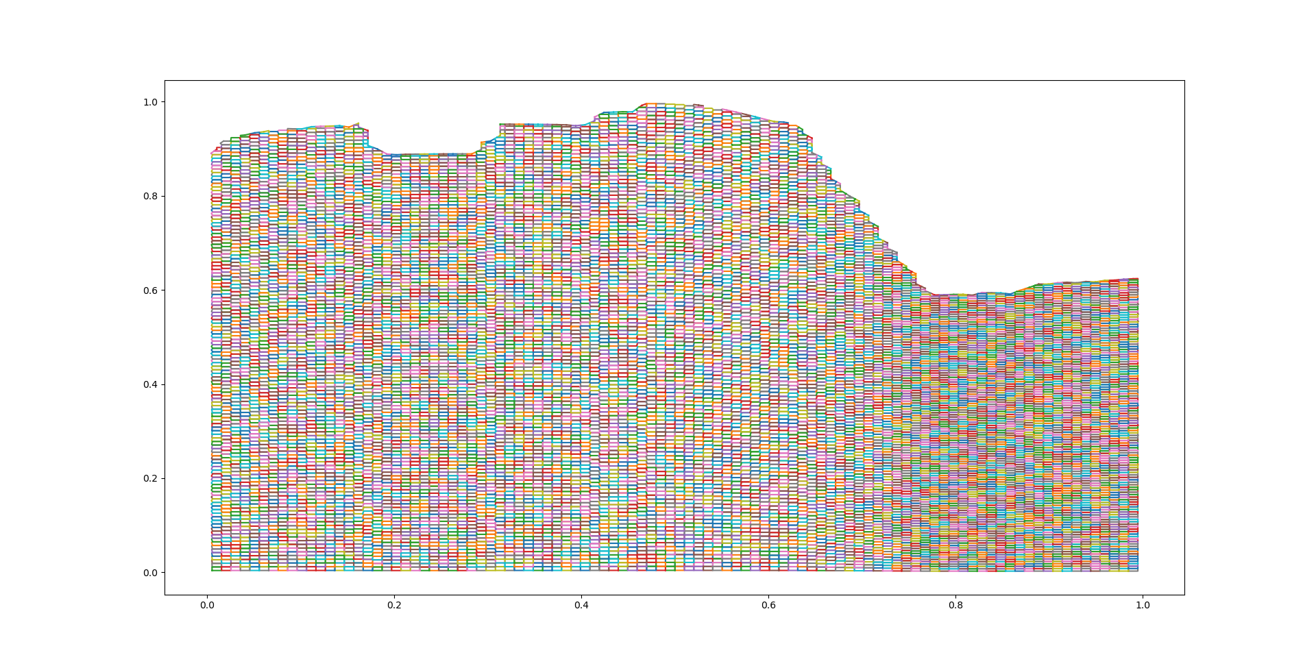
Step 3.1 : Create Voronoi regions and polygonize them

In this step the Voronoi regions are created to facilitate the clustering. These regions are turned into polygons that can be clustered and merged efficiently. In the following plot the resulting polygons are plotted.

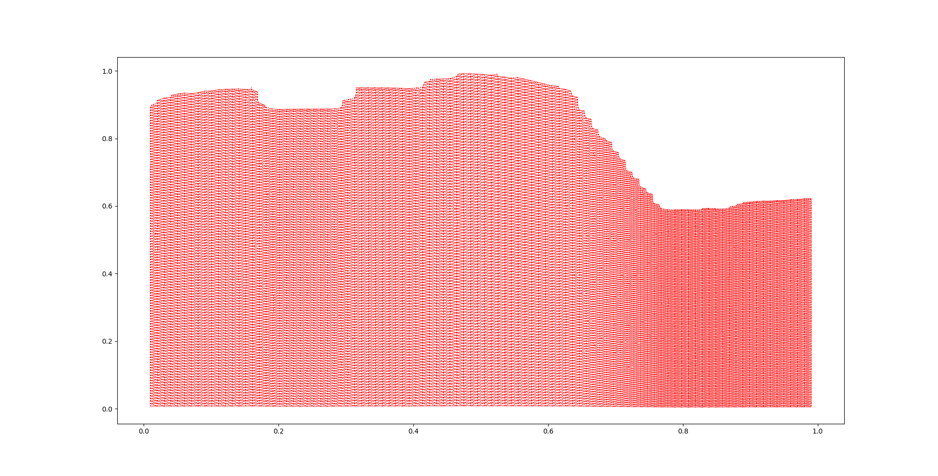
Step 3.1 : Create the spatial connectivity matrix

The polygons shown in the figure above will be used to construct a connectivity weight matrix. The weight matrix will be used as a “guide” from the clustering method. Different spatial weight matrix methods can be found in the libpysal website ( https://pysal.org/libpysal/api.html )

Using the Queen method, the adjacency relationships can be visualized in the following graph we can observe that every polygon is essentially only connected to the polygons that are next to it.

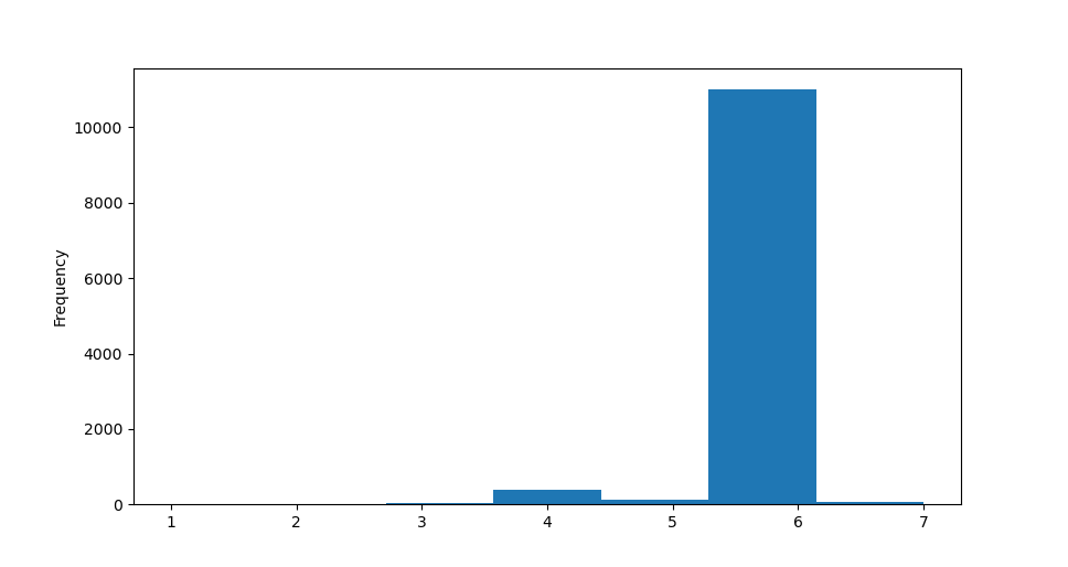
This claim is further supported by the fact that the neighboring polygons are ranging between 3 and 7, with 6 being the most common number of neighbors.

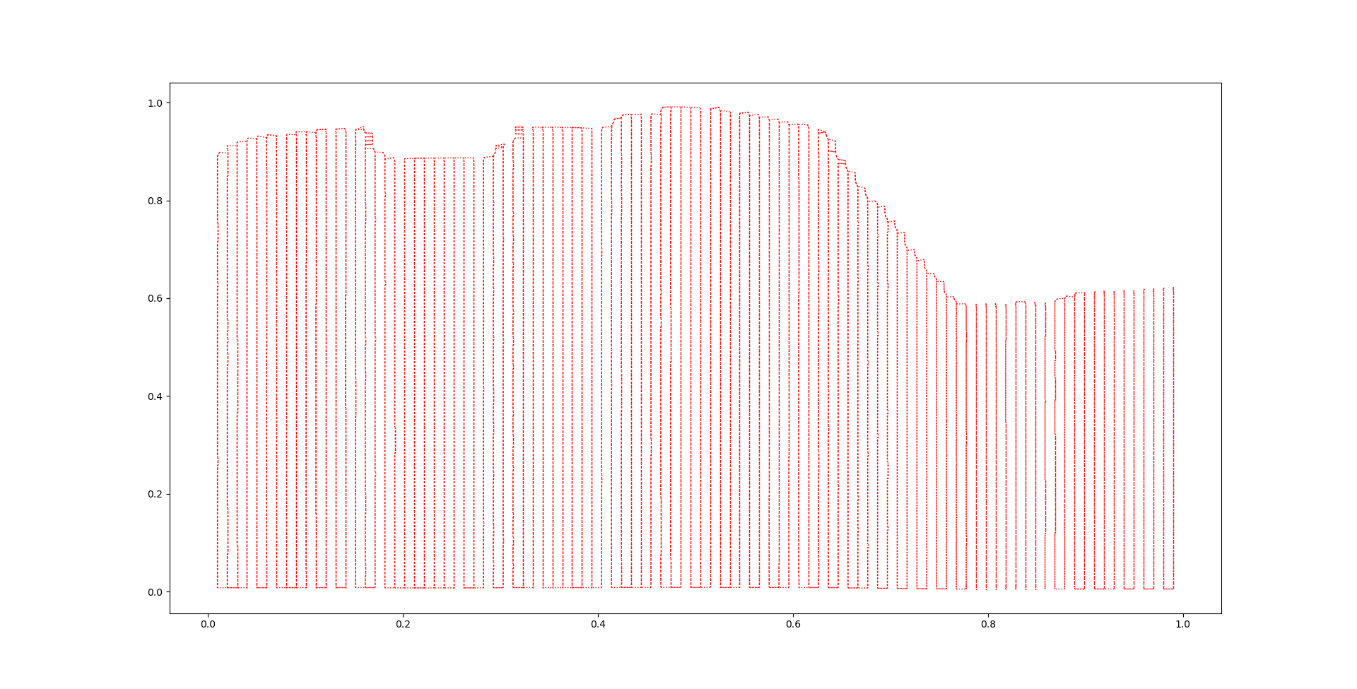
Using the KNN method and the clustering inputs of the x, y and IC value, we observe that the connectivity matrix is biased towards the y dimension.

Step 3.1 : Perform the clustering using the Agglomerative Clustering method

In this method we use the Agglomerative Clustering method as clustering method because the weight matrix can be used as input. In this case with 4 clusters used this leas to the following results

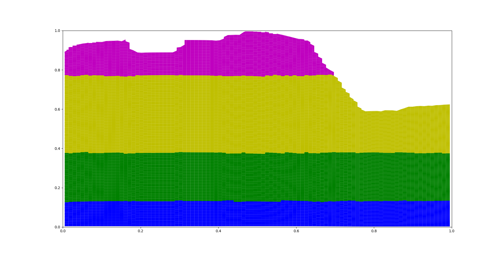
Step 4: Polygons are created by merging clusters

The small polygons are grouped by each cluster group and they are merged together.

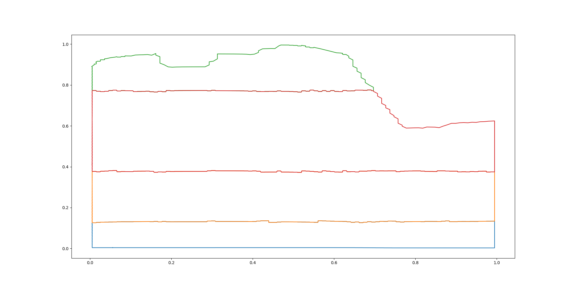
Step 5: Polygons are simplified

The polygons are simplified by using the Douglas-Peucker algorithm.

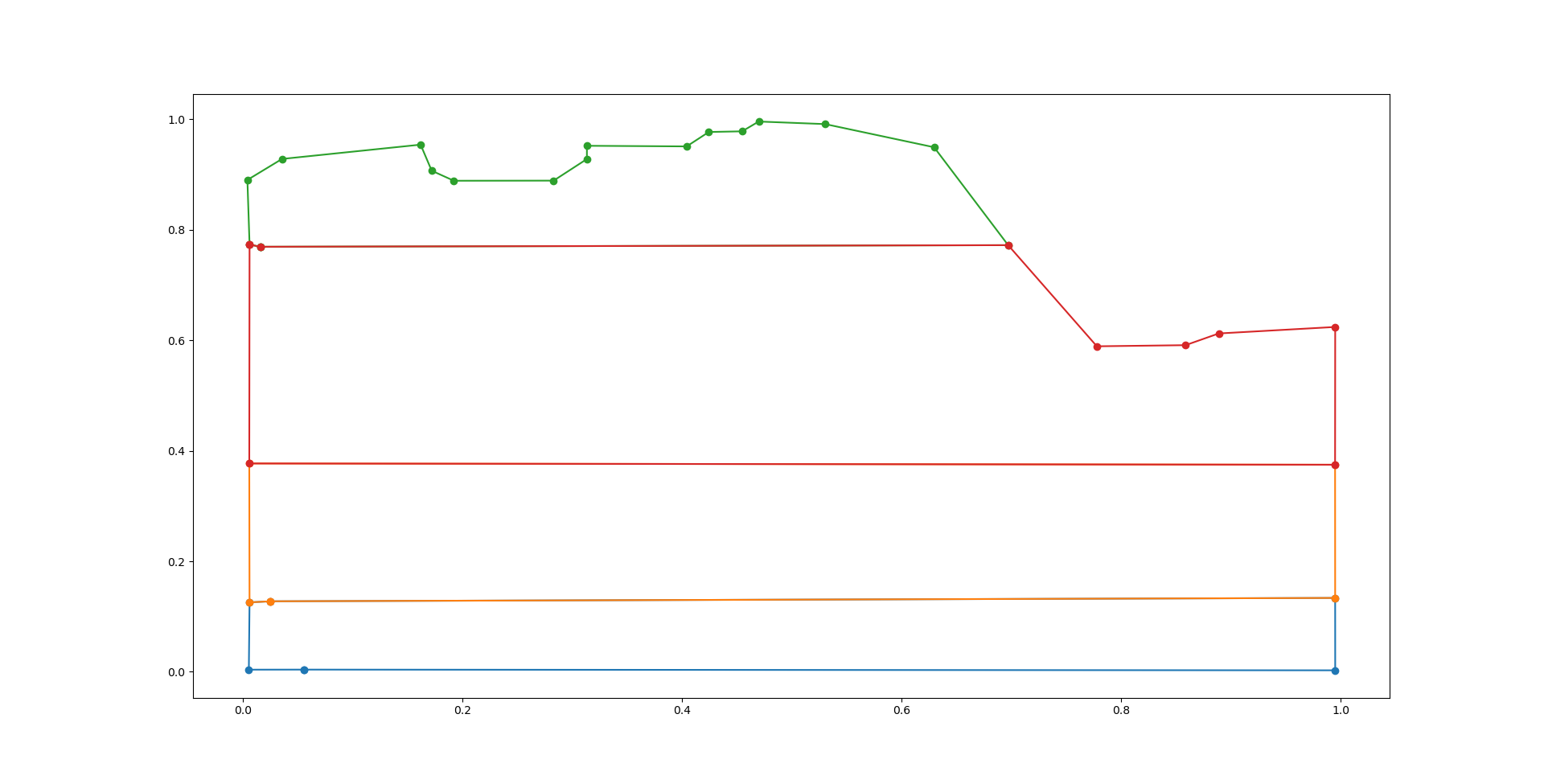
Step 6: IC values per polygon are extracted

The mean and standard deviation of the points included in the polygon are extracted.