How to get a 2d interpolated slice from a list of data

In this tutorial the user will learn how to extract a 2d interpolated slice. The first step is to import all relevant packages needed for the tutorial.

import numpy as np
from matplotlib import pyplot as plt
from mpl_toolkits.mplot3d import Axes3D
import pickle

from datafusiontools._core.data_input import Data, Geometry, Variable
from datafusiontools.interpolation.interpolation_2d_slice import Interpolate2DSlice
from datafusiontools.interpolation.interpolation import Nearest
from datafusiontools.spatial_utils.ahn_utils import SpatialUtils

In this example the data will be interpolated using the Nearest Neighbor model. However the user can use any of the interpolation models included in DataFusionTools or implement their own.

The data were stored in a pickle file. The pickle file can be opened as follows using python.

input_files = "test_case_DF.pickle"
with open(input_files, "rb") as f:
    (cpts, resistivity, insar) = pickle.load(f)

After all data are extracted from the pickle file, they will be reorganized into lists of datafusiontools._core.data_input.Data The cpts are extracted in the following way:

cpts_list = []
for name, item in cpts.items():
    location = Geometry(x=item["coordinates"][0], y=item["coordinates"][1], z=0)
    cpts_list.append(
        Data(
            location=location,
            independent_variable=Variable(value=item["NAP"], label="NAP"),
            variables=[
                Variable(value=item["water"], label="water"),
                Variable(value=item["tip"], label="tip"),
                Variable(value=item["IC"], label="IC"),
                Variable(value=item["friction"], label="friction"),
            ],
        )
    )

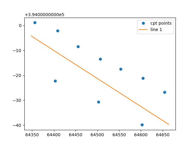
After all the data is organized the user must select two points in the x-y plane which will be used as boundaries of the 2d slice. The two locations are defined by using the datafusiontools._core.data_input.Geometry class. The locations selected for this example can be seen bellow.

location_1 = Geometry(x=64348.1, y=393995.8, z=0)
location_2 = Geometry(x=64663.8, y=393960.3, z=0)

The following image shows the location of the 2d slice to be extracted.

Then the class DataFusionTools.interpolation.interpolation_2d_slice.Interpolate2DSlice.get_2d_slice_extra() class can be initialized and the function.

interpolator = Interpolate2DSlice()
points_2d_slice, results_2d_slice = interpolator.get_2d_slice_extra(
    location_1=location_1,
    location_2=location_2,
    data=cpts_list,
    interpolate_variable="IC",
    number_of_points=100,
    number_of_independent_variable_points=120,
    interpolation_method=Nearest()
)

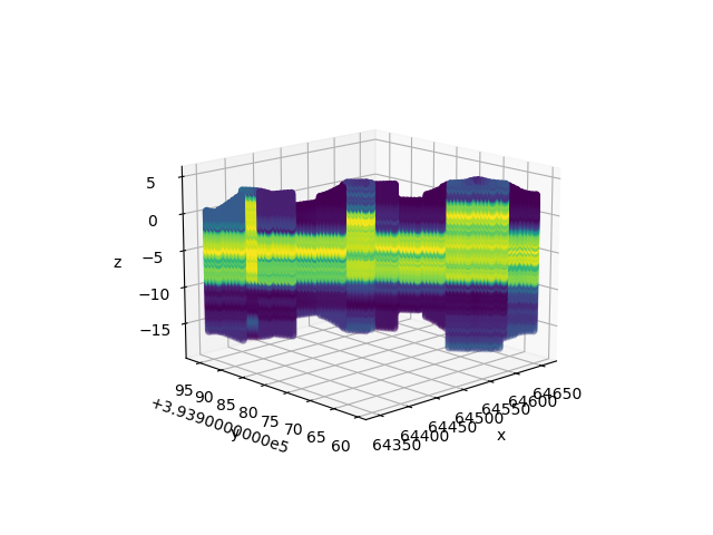
To view the results the user can create a plot function as the one appended bellow.

fig = plt.figure()
ax = fig.add_subplot(111, projection="3d")
ax.set_xlabel("x")
ax.set_ylabel("y")
ax.set_zlabel("z")
for counter, points in enumerate(points_2d_slice):
    values = results_2d_slice[counter]
    ax.scatter(
        np.array(points).T[0],
        np.array(points).T[1],
        np.array(points).T[2],
        c=values,
    )

Which produces the following figure.

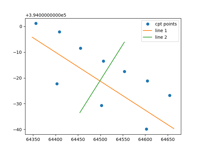
We can also choose a second slice with the same data. The line can be redefined as it can be seen bellow.

location_1 = Geometry(x=64454.3, y=393966.5, z=0)
location_2 = Geometry(x=64553.6, y=393993.9, z=0)

The following image shows the locations the first and second 2d slices to be extracted.

The function DataFusionTools.interpolation.interpolation_2d_slice.Interpolate2DSlice.get_2d_slice_extra() has to be called again as it can be seen in the following snippet.

points_2d_slice, results_2d_slice = interpolator.get_2d_slice_extra(
    location_1=location_1,
    location_2=location_2,
    data=cpts_list,
    interpolate_variable="IC",
    number_of_points=100,
    number_of_independent_variable_points=120,
    interpolation_method=Nearest()
)

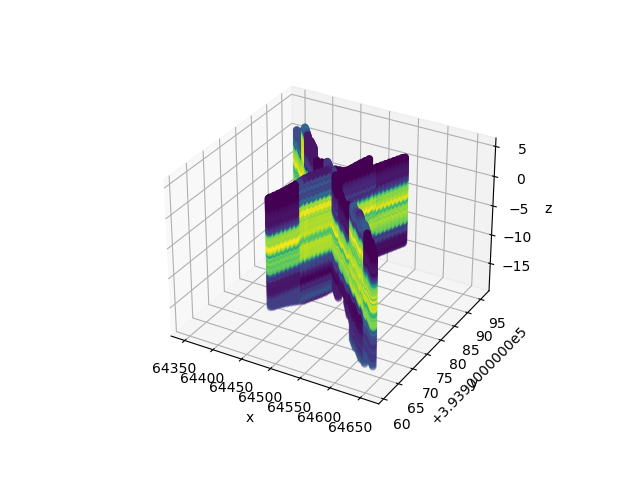
The results of the last slice can be added in the previously created plot.

for counter, points in enumerate(points_2d_slice):
    values = results_2d_slice[counter]
    ax.scatter(
        np.array(points).T[0],
        np.array(points).T[1],
        np.array(points).T[2],
        c=values,
    )

plt.show()

Which produces the following figure.

Note that the user can also input their own surface line in the in the DataFusionTools.interpolation.interpolation_2d_slice.Interpolate2DSlice.get_2d_slice_extra() function. For example the user can use the functionality of extracting surfaces from the AHN and using those set of points as an input. The points are extracted from the DTM map of the AHN. Note values that are larger that +323m and smaller than -7m are filtered out of the data.

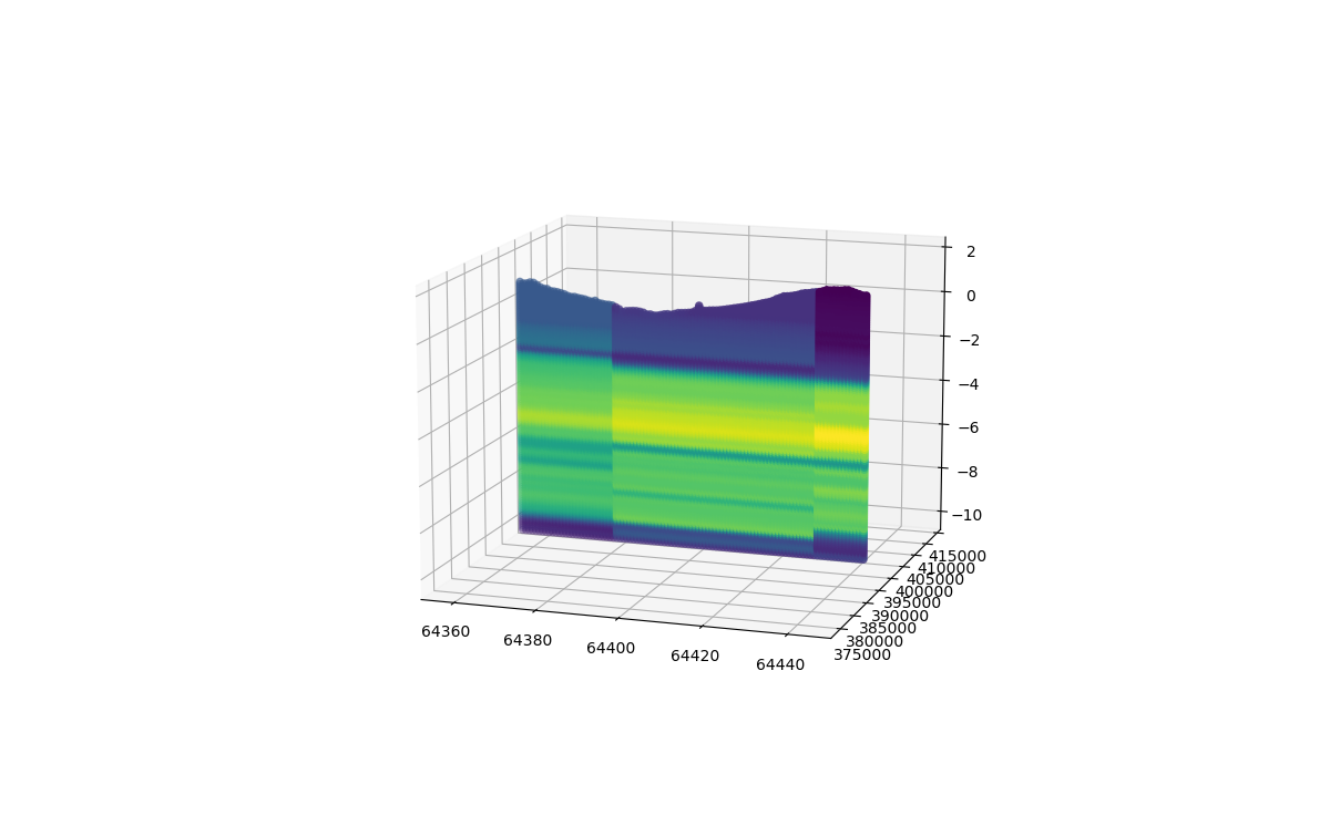
In the following code snippet the locations of the slice are defined. As well as the surface line that is extracted from the AHN.

location_1 = Geometry(x=64358.1, y=393995, z=0)
location_2 = Geometry(x=64443.8, y=393995, z=0)
spacial_utils = SpatialUtils()
surface_line = []
for i in np.arange(location_1.x,location_2.x,  1):
    surface_line.append([i, location_1.y])
surface_line = np.array(spacial_utils.get_ahn_surface_line(np.array(surface_line)))

The bottom line can be defined as a horizontal line at -10m.

bottom_line =  np.array([[location_1.x, location_1.y, -10], [location_2.x, location_2.y, -10]])

The same function is called as in the case above.

points_2d_slice, results_2d_slice = interpolator.get_2d_slice_extra(
    location_1=location_1,
    location_2=location_2,
    data=cpts_list,
    interpolate_variable="IC",
    number_of_points=100,
    number_of_independent_variable_points=120,
    top_surface=surface_line,
    bottom_surface=bottom_line
)

Which produces the following figure.